
Conditional Formatting in Excel with Formula Current Cell

What to Put into Formula to Determine Conditional Formatting to Reference Current Cell? E. G. I Want to Make Conditional Formatting for If Cell Contains Error...
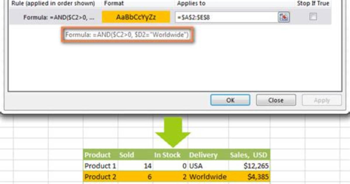
What to put into formula to determine conditional formatting to reference current cell? E.g. I want to make conditional formatting for if cell contains error (#N/A) and use the same rule for the entire column.
Cant seem to find how to reference the cell for which the function is being evaluated. Is it even possible?
3 Answers
Suppose the data range to conditionally format is A2:A10.
- Select first cell
A2. - From Home TAB, Click Conditional Formatting, Manage Rules, New Rule.
- Under use formula to determine which cell to format. In the field Format
values where this formula is true, enter
=ISNA($A2). - Click Format to set the cell formatting, then select OK.
- In the Conditional Formatting Rules Manager, edit the range under
Applies to set
$A2:$A10. - Select Apply then OK.
Must Read
Using relative references to refer to the current cell
In a conditional formatting formula, you can refer to the current cell by using the relative form of its usual address. e.g. If you want to format cell B2, then you could use a formula like this:
=ISNA(B2)
Because you use a relative reference (B2 rather than $B$2), when you copy it to a different cell, the formula is adjusted to be relative to the new cell. So if you use the format painter to copy the conditional format to cell C3 (or just copy the whole of B2 there), then inspect C3 in the conditional formatting rules manager, then you will see that the formula has automatically updated to
=ISNA(C3)
This principle also applies to ranges, but is a little trickier to understand. For a range, the formula is input relative to the top-left cell, but is interpreted relative to each cell in turn. So if you select the range of cells from B2 to D4, and apply the formula =ISNA(B2), any cell in the range will be formatted if it contains #N/A, not just B2.
Elena Rostova holds a Master's degree in Public Health Journalism. She covers groundbreaking medical research, holistic wellness trends, mental health awareness, and nutritional science.
