
Creating a Density Histogram in Ggplot2?

I Want to Create the Next Histogram Density Plot with Ggplot2. in the "Normal" Way (Base Packages) Is Really Easy: Set. Seed(46) Vector
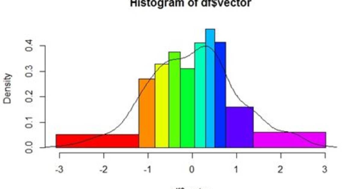
I want to create the next histogram density plot with ggplot2. In the "normal" way (base packages) is really easy:
set.seed(46)
vector <- rnorm(500)
breaks <- quantile(vector,seq(0,1,by=0.1))
labels = 1:(length(breaks)-1)
den = density(vector)
hist(df$vector,
     breaks=breaks,
     col=rainbow(length(breaks)),
     probability=TRUE)
lines(den)
With ggplot I have reached this so far:
seg <- cut(vector,breaks,
           labels=labels,
           include.lowest = TRUE, right = TRUE)
df = data.frame(vector=vector,seg=seg)

ggplot(df) +
     geom_histogram(breaks=breaks,
                    aes(x=vector,
                        y=..density..,
                        fill=seg)) +
     geom_density(aes(x=vector,
                      y=..density..))
But the "y" scale has the wrong dimension. I have noted that the next run gets the "y" scale right.
 ggplot(df) +
     geom_histogram(breaks=breaks,
                    aes(x=vector,
                    y=..density..,
                    fill=seg)) +
     geom_density(aes(x=vector,
                      y=..density..))
I just do not understand it. y=..density.. is there, that should be the height. So why on earth my scale gets modified when I try to fill it?
I do need the colours. I just want a histogram where the breaks and the colours of each block are directionally set according to the default ggplot fill colours.
4 Answers
Manually, I added colors to your percentile bars. See if this works for you.
library(ggplot2)

ggplot(df, aes(x=vector)) +
   geom_histogram(breaks=breaks,aes(y=..density..),colour="black",fill=c("red","orange","yellow","lightgreen","green","darkgreen","blue","darkblue","purple","pink")) +
   geom_density(aes(y=..density..)) +
   scale_x_continuous(breaks=c(-3,-2,-1,0,1,2,3)) +
   ylab("Density") + xlab("df$vector") + ggtitle("Histogram of df$vector") +
   theme_bw() + theme(plot.title=element_text(size=20),
                      axis.title.y=element_text(size = 16, vjust=+0.2),
                      axis.title.x=element_text(size = 16, vjust=-0.2),
                      axis.text.y=element_text(size = 14),
                      axis.text.x=element_text(size = 14),
                      panel.grid.major = element_blank(),
                      panel.grid.minor = element_blank())
fill=seg results in grouping. You are actually getting a different histogram for each value of seg. If you don't need the colours, you could use this:
ggplot(df) +
  geom_histogram(breaks=breaks,aes(x=vector,y=..density..), position="identity") +
  geom_density(aes(x=vector,y=..density..))
If you need the colours, it might be easiest to calculate the density values outside of ggplot2.
Or an option with ggpubr
library(ggpubr)
gghistogram(df, x = "vector", add = "mean", rug = TRUE, fill = "seg",
   palette = c("#00AFBB", "#E7B800", "#E5A800", "#00BFAB", "#01ADFA",
   "#00FABA", "#00BEAF", "#01AEBF", "#00EABA", "#00EABB"), add_density = TRUE)
The confusion regarding interpreting the y-axis might be due to density is plotted rather than count. So, the values on the y-axis are proportions of the total sample, where the sum of the bars is equal to 1.
Marcus Vance is a cybersecurity auditor and technology writer dedicated to educating the public about online safety, data privacy regulations, enterprise security, and emerging cyber threats.
