
Derive the Gradient Through Torch. Topk

I Want to Derive the Gradient Through Torch. Topk Function. Suppose I the Input Is a Vector, Then It Is Transformed by a Parameter Matrix, and the Top K Values...
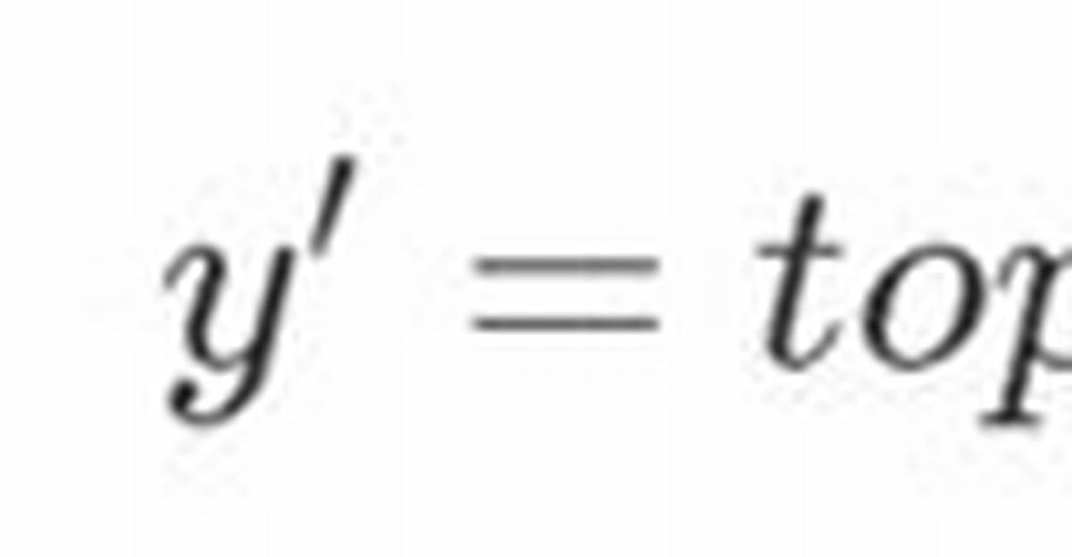
I want to derive the gradient through torch.topk function.
Suppose I the input is a vector ,
then it is transformed by a parameter matrix ,
and the top k values of the vector are selected .
The result vector is further transformed by element-wise multiplication.
Finally the loss is computed by
.
I wonder, is the loss differentiable with respect to W? Formally, can we calculate the following gradient?
2 Answers
The topk() operation is simply a linear transformation to pick the top k elements of a tensor. Since this is a W @ X or matrix-vector multiplication kind of operation, this is also differentiable.
Example: Below I have computed the pipelined operation topk(Wx) in two ways and showed the gradients resulting from both are identical.
In [1]: import torch

In [2]: x1 = torch.rand(6, requires_grad = True)

In [3]: W1 = torch.rand(6, 6, requires_grad = True)

In [4]: x1
Out[4]: tensor([0.1511, 0.5990, 0.6338, 0.5137, 0.5203, 0.0560], requires_grad=True)

In [5]: W1
Out[5]:
tensor([[0.2541, 0.6699, 0.5311, 0.7801, 0.5042, 0.5475],
        [0.7523, 0.1331, 0.7670, 0.8132, 0.0524, 0.0269],
        [0.3974, 0.2880, 0.9142, 0.9906, 0.4401, 0.3984],
        [0.7956, 0.2071, 0.2209, 0.6192, 0.2054, 0.7693],
        [0.8587, 0.8415, 0.6033, 0.3812, 0.2498, 0.9813],
        [0.9033, 0.0417, 0.2272, 0.1576, 0.9087, 0.3284]], requires_grad=True)

In [6]: y1 = W1 @ x1

In [7]: y1
Out[7]: tensor([1.4699, 1.1260, 1.5721, 0.8523, 1.3969, 0.8776], grad_fn=<MvBackward>)

In [8]: yk, _ = torch.topk(y1, 3)

In [9]: yk
Out[9]: tensor([1.5721, 1.4699, 1.3969], grad_fn=<TopkBackward>)

In [10]: loss1 = (yk ** 2).sum()

In [11]: loss1.backward()

In [12]: W1.grad
Out[12]:
tensor([[0.4442, 1.7609, 1.8633, 1.5102, 1.5296, 0.1646],
        [0.0000, 0.0000, 0.0000, 0.0000, 0.0000, 0.0000],
        [0.4751, 1.8833, 1.9928, 1.6152, 1.6359, 0.1760],
        [0.0000, 0.0000, 0.0000, 0.0000, 0.0000, 0.0000],
        [0.4222, 1.6734, 1.7706, 1.4352, 1.4535, 0.1564],
        [0.0000, 0.0000, 0.0000, 0.0000, 0.0000, 0.0000]])
Now let us evaluate the same set of operations but using topk() as a linear transformation explicitly. Note that the constructed Wk matrix selectively picks out top k (here 3) elements from the 6 element tensor through multiplication.
In [13]: x2 = torch.tensor([0.1511, 0.5990, 0.6338, 0.5137, 0.5203, 0.0560], req
    ...: uires_grad=True)

In [14]: W2 = torch.tensor([[0.2541, 0.6699, 0.5311, 0.7801, 0.5042, 0.5475],
    ...:         [0.7523, 0.1331, 0.7670, 0.8132, 0.0524, 0.0269],
    ...:         [0.3974, 0.2880, 0.9142, 0.9906, 0.4401, 0.3984],
    ...:         [0.7956, 0.2071, 0.2209, 0.6192, 0.2054, 0.7693],
    ...:         [0.8587, 0.8415, 0.6033, 0.3812, 0.2498, 0.9813],
    ...:         [0.9033, 0.0417, 0.2272, 0.1576, 0.9087, 0.3284]], requires_gra
    ...: d=True)

In [15]: y2 = W2 @ x2

In [16]: y2
Out[16]: tensor([1.4700, 1.1260, 1.5721, 0.8523, 1.3969, 0.8776], grad_fn=<MvBackward>)

# Use the indices obtained earlier to construct the matrix
In [19]: _
Out[19]: tensor([2, 0, 4])

In [20]: k = 3

In [21]: Wk = torch.zeros(k, y2.shape[0])

In [22]: Wk[torch.arange(k), _] = 1

In [23]: Wk.requires_grad = True

In [24]: Wk
Out[24]:
tensor([[0., 0., 1., 0., 0., 0.],
        [1., 0., 0., 0., 0., 0.],
        [0., 0., 0., 0., 1., 0.]], requires_grad=True)


In [25]: yk2 = Wk @ y2

In [26]: yk2
Out[26]: tensor([1.5721, 1.4700, 1.3969], grad_fn=<MvBackward>)

In [27]: loss2 = (yk2 ** 2).sum()

In [28]: loss2.backward()
Now compare the gradients obtained in both cases:
In [29]: W2.grad
Out[29]:
tensor([[0.4442, 1.7611, 1.8634, 1.5103, 1.5297, 0.1646],
        [0.0000, 0.0000, 0.0000, 0.0000, 0.0000, 0.0000],
        [0.4751, 1.8834, 1.9929, 1.6152, 1.6360, 0.1761],
        [0.0000, 0.0000, 0.0000, 0.0000, 0.0000, 0.0000],
        [0.4222, 1.6735, 1.7707, 1.4352, 1.4536, 0.1565],
        [0.0000, 0.0000, 0.0000, 0.0000, 0.0000, 0.0000]])

In [30]: W1.grad
Out[30]:
tensor([[0.4442, 1.7609, 1.8633, 1.5102, 1.5296, 0.1646],
        [0.0000, 0.0000, 0.0000, 0.0000, 0.0000, 0.0000],
        [0.4751, 1.8833, 1.9928, 1.6152, 1.6359, 0.1760],
        [0.0000, 0.0000, 0.0000, 0.0000, 0.0000, 0.0000],
        [0.4222, 1.6734, 1.7706, 1.4352, 1.4535, 0.1564],
        [0.0000, 0.0000, 0.0000, 0.0000, 0.0000, 0.0000]])

In [31]: x1.grad
Out[31]: tensor([4.3955, 5.2256, 6.1213, 6.4732, 3.5637, 5.6037])

In [32]: x2.grad
Out[32]: tensor([4.3957, 5.2261, 6.1215, 6.4733, 3.5641, 5.6040])
As you can see the results are identical upto some floating point errors which were introduced when I copied the values of x1 and W1 without taking their full precision.
I figured it out thanks to @swag2198 and I posted the formulation on my repository
Sarah Jenkins is a veteran tech journalist with over 12 years of experience covering artificial intelligence, mobile innovations, and digital ethics. Her insights have appeared in leading technology publications worldwide.
