
How to Create Graph Using Pivot Table in Excel

How Do You Create a Pivot Chart with Selected Data? Pivotcharts Select Any Cell in Your Pivottable. Clicking a Cell in the Pivottable. from the Insert Tab...
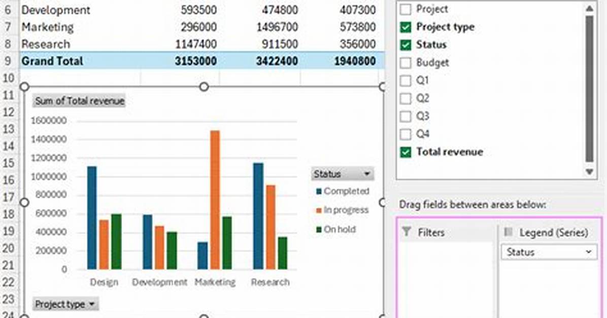
How do you create a pivot chart with selected data?
PivotCharts
- Select any cell in your PivotTable. Clicking a cell in the PivotTable.
- From the Insert tab, click the PivotChart command. Clicking the PivotChart command.
- The Insert Chart dialog box will appear. Select the desired chart type and layout, then click OK.
- The PivotChart will appear. The inserted PivotChart.
What is the difference between Pivot Table and Pivot Chart?
Pivot Tables allow you to create a powerful view with data summarized in a grid, both in horizontal and vertical columns (also known as Matrix Views or Cross Tabs). A Pivot Chart is an interactive graphical representation of the data in your Zoho Creator application.
What is the purpose of creating a pivot chart from your pivot table?
Pivot charts let you rapidly analyze large amounts of unsummarized data in different ways. Unlike normal charts, Pivot charts can be used to plot data with hundreds or thousands of rows.
What is purpose of pivot table?
Pivot tables are a technique in data processing. They arrange and rearrange (or “pivot“) statistics in order to draw attention to useful information. This leads to finding figures and facts quickly making them integral to data analysis.
Why do we need pivot chart?
A Pivot Table is used to summarise, sort, reorganise, group, count, total or average data stored in a table. It allows us to transform columns into rows and rows into columns. It allows grouping by any field (column), and using advanced calculations on them.
How do I make a pivot chart?
Select a cell in your PivotTable. On the Insert tab, select the Insert Chart dropdown menu, and then click any chart option. The chart will now appear in the worksheet.
Create a chart from a PivotTable
- Select a cell in your table.
- Select PivotTable Tools > Analyze > PivotChart .
- Select a chart.
- Select OK.
How do you pivot?
To insert a pivot table, execute the following steps.
- Click any single cell inside the data set.
- On the Insert tab, in the Tables group, click PivotTable. The following dialog box appears. Excel automatically selects the data for you. The default location for a new pivot table is New Worksheet.
- Click OK.
How do you create a pivot table for dummies?
How to Create a Pivot Table
- Enter your data into a range of rows and columns.
- Sort your data by a specific attribute.
- Highlight your cells to create your pivot table.
- Drag and drop a field into the “Row Labels” area.
- Drag and drop a field into the “Values” area.
- Fine-tune your calculations.
What is shortcut key of pivot table?
Pivot Table Keyboard Shortcuts Reference Chart
| Shortcut | Action |
|---|---|
| Ctrl + Shift + * | Select entire pivot table (not including Report Filters) |
| Ctrl + A | Select entire pivot table (not including Report Filters) |
| Spacebar | Add or remove checkmark for selected field in PivotTable Field List |
•
Mar 3, 2021
What is pivot table and pivot chart in Excel?
What is an Excel Pivot Table and Chart? A pivot table is a program tool, that is a built-in feature of MS Excel, allowing you to organize and summarize selected columns and rows of data in a spreadsheet to obtain a desired report, helping in visualization of data.
What is an Excel pivot table report?
An Excel PivotTable is a tool to explore and summarize large amounts of data, analyze related totals and present summary reports designed to: Rotate rows to columns or columns to rows (which is called “pivoting”) to view different summaries of the source data.
What is Pivot Chart explain?
Pivot Chart in excel is an in-built Programme tool in excel which helps you out to summarize selected rows and column of data in a spreadsheet. It’s the visual representation of a pivot table or any tabular data which helps to summarize & analyze the datasets, patterns, and trends.
What does pivot mean?
: the action of turning around a point : the action of pivoting. : a person or thing that is central or important to someone or something else.
What is the benefit of pivot table in Excel?
Pivot Tables are worksheet tables that let you summarize and analyze your Excel data. Benefits include: Ability to recap using any data element and then drill down to review the details. Formulas may restrict sorting capabilities or may be corrupted when adding and deleting rows or columns.
How do I change the type of pivot chart?
Change the style of your PivotTable
- Click anywhere in the PivotTable to show the PivotTable Tools on the ribbon.
- Click Design, and then click the More button in the PivotTable Styles gallery to see all available styles.
- Pick the style you want to use.
- If you don’t see a style you like, you can create your own.
How do you manipulate a pivot table?
What are the four primary areas of a PivotTable?
In it are four areas (Filters, Columns, Rows, and Values) where various field names can be placed to create a PivotTable.
Can you hide pivot tables?
When using a data model for a Power View or PivotTable report, you can hide entire tables or individual columns so that only relevant items appear in the field list. To hide an entire table, right-click the tab that contains the table and choose Hide from Client Tools.
Can you filter pivot table?
In the PivotTable, select one or more items in the field that you want to filter by selection. Right-click an item in the selection, and then click Filter. Do one of the following: Right-click another item in the same field, click Filter, and then click Clear Filter.
David Miller brings 15 years of experience in global economics, personal finance strategy, and market dynamics. He specializes in turning complex economic trends into actionable insights for everyday readers.
