
How to Create Pivot Table in Excel Mac

How Do I Create a Pivot Table in Excel 2016 for Mac? Highlight the Cell Where You’d Like to Create the Pivot Table. in This Example, We’ve Selected Cell A1 on...
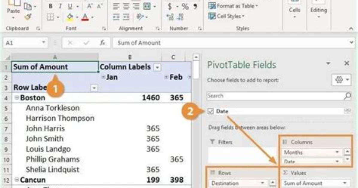
How do I create a pivot table in Excel 2016 for Mac?
How do you use pivot tables on a Mac?
Select your data table, then click Insert on the toolbar and then Recommended PivotTables in the Insert tab that appears. Excel will automatically create a meaningful layout on a new sheet based on your source data.
Where is the pivot chart in Excel for Mac?
How do I make a pivot table in Mac numbers?
What is pivoting in Excel?
How do you add a filter on numbers?
How do you create a filter in numbers?
- Select any cell within the range.
- Select Data > Filter.
- Select the column header arrow .
- Select Text Filters or Number Filters, and then select a comparison, like Between.
- Enter the filter criteria and select OK.
How do you sort A to Z in numbers?
How do I sort data in Mac numbers?
Do numbers or symbols go first in alphabetical order?
So your system will start with numerical headers. If you’re using an alphabetical system, you’ll file numbers in ascending order, that is smallest to largest, the same way you would proceed through the alphabet.
How do I sort data in numbers?
- Tap the table, then tap the letter above the column with the data you want to sort by.
- Tap. at the bottom of the screen, then tap an option: Sort Ascending: Sorts the table rows in alphabetical order (A to Z) or by increasing numerical values based on the data in the selected column.
How do I sort numbers in sheets?
How do I rearrange columns in numbers?
How do I sort a list of numbers in Excel?
- Select a single cell in the column you want to sort.
- On the Data tab, in the Sort & Filter group, click. to perform an ascending sort (from A to Z, or smallest number to largest).
- Click. to perform a descending sort (from Z to A, or largest number to smallest).
Can Excel put numbers in order?
How do I automatically number rows in Excel?
- In the first cell of the range that you want to number, type =ROW(A1). The ROW function returns the number of the row that you reference. For example, =ROW(A1) returns the number 1.
- Drag the fill handle. across the range that you want to fill.
How do I automatically number rows in Excel without dragging?
- Enter 1 in cell A1.
- Go to Home –> Editing –> Fill –> Series.
- In the Series dialogue box, make the following selections: Series in: Columns. Type: Linear. Step Value: 1. Stop Value: 1000.
- Click OK.
How do I automatically number rows in numbers?
What is the formula to count rows in Excel?
- Select the cell in which you want to see the count (cell A12 in this example)
- Type a formula to count rows greater than or equal to 5: =COUNTIF(B1:B10,”>=5″)
- Type a minus sign.
- Type a formula to count rows greater than 10:
- The completed formula is:
- Press the Enter key to complete the entry.
How do you count entries in Excel?
How do I count the number of cells with text?
Robert Thorne covers electric vehicle innovations, autonomous driving systems, global mobility trends, and automotive engineering developments.
