
How to Implement Averaged Perceptron in Python (Without Scikit-Learn)

I Am Trying to Fit the Binary Classification Using Averaged Perceptron Model. I Followed the Instructions Line by Line of the Book by Daume () (Page 53 for...
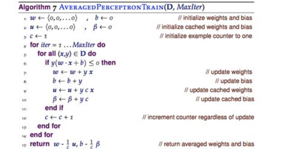
I am trying to fit the binary classification using Averaged Perceptron model.
I followed the instructions line by line of the book by Daume
() (Page 53 for averaged perceptron).
Here is my implementation:
def aperceptron_sgd(X, Y,epochs):
    # initialize weights
    w = u = np.zeros(X.shape[1] )
    b = beta = 0

    # counters
    final_iter = epochs
    c = 1
    converged = False

    # main average perceptron algorithm
    for epoch in range(epochs):
        # initialize misclassified
        misclassified = 0

        # go through all training examples
        for  x,y in zip(X,Y):
            h = np.dot(x, w)*y

            if h <= 0:
                w = w + y*x
                b = b + y

                u = u+ y*c*x
                beta = beta + y*c
                misclassified += 1

        # update counter regardless of good or bad classification
        c = c + 1

        # break loop if w converges
        if misclassified == 0:
            final_iter = epoch
            converged = True
            print("Averaged Perceptron converged after: {} iterations".format(final_iter))
            break

    if converged == False:
        print("Averaged Perceptron DID NOT converged.")

    # prints
    # print("final_iter = {}".format(final_iter))
    # print("b, beta, c , (b-beta/c)= {} {} {} {}".format(b, beta, c, (b-beta/c)))
    # print("w, u, (w-u/c) {} {} {}".format(w, u, (w-u/c)) )


    # return w and final_iter
    w = w - u/c
    b = np.array([b- beta/c])
    w = np.append(b, w)

    return w, final_iter
However, When I test this with the data it gives inaccurate predictions.
The data is given here:
 1.36  3.57     1
 1.78 -0.79    -1
-0.88  0.96     1
 1.64 -0.63    -1
-0.98  1.34     1
 1.50  0.33    -1
 0.15  1.48     1
 1.39 -1.71    -1
 0.08  2.24     1
 1.87 -0.35    -1
 0.25  2.52     1
 1.68 -0.56    -1
 0.23  2.75     1
 2.05 -0.85    -1
-0.53  1.40     1
 1.92 -0.60    -1
 0.12  2.77     1
 1.70 -0.40    -1
 0.72  2.01     1
 0.44 -0.51    -1
-1.84  1.13     1
 1.46  1.65    -1
 0.48  1.94     1
 1.57 -0.22    -1
-0.45  2.14     1
 2.71 -0.19    -1
-1.04  1.82     1
 2.56  0.49    -1
 0.26  2.29     1
 1.51 -1.11    -1
 0.27  1.36     1
 2.99  0.84    -1
 0.37  2.89     1
 2.81  0.19    -1
-0.48  1.23     1
 2.12 -0.26    -1
-0.46  0.47     1
 0.77 -0.65    -1
 1.52  2.75     1
 4.01  1.79    -1
 0.67  2.24     1
 1.75  0.52    -1
 0.19  1.80     1
 2.61  0.44    -1
-0.54  0.36     1
 0.67 -0.59    -1
 0.71  2.94     1
 1.82 -0.99    -1
 0.88  3.82     1
 0.78 -1.33    -1
 1.17  2.82     1
 2.17  0.46    -1
 1.05  2.52     1
 0.71 -1.14    -1
-0.25  2.07     1
 1.77  0.29    -1
 0.33  3.12     1
 0.37 -2.22    -1
 0.35  1.79     1
 1.10  0.71    -1
 0.73  2.74     1
 2.26 -0.93    -1
-0.20  1.81     1
 1.07 -1.21    -1
 1.70  3.04     1
 2.86  1.26    -1
-0.75  1.72     1
 2.38  0.12    -1
-0.41  0.69     1
 2.19  0.71    -1
 1.42  3.66     1
 1.50  0.46    -1
 0.50  2.06     1
 1.84 -0.46    -1
-1.53  0.12     1
 0.78 -0.52    -1
-0.21  0.96     1
 3.54  2.02    -1
-0.14  1.16     1
 2.09  0.39    -1
-0.79  1.64     1
 0.75  0.47    -1
 1.02  3.60     1
 0.07 -1.45    -1
-0.79  1.48     1
 2.75  0.24    -1
-0.10  1.92     1
 1.99  0.31    -1
 0.86  2.10     1
 2.49 -0.05    -1
 1.31  3.54     1
 1.04 -1.65    -1
-1.45  0.31     1
 1.75 -1.01    -1
-1.53  0.47     1
 2.13 -0.42    -1
 0.06  2.06     1
 2.20 -0.40    -1
 0.94  1.37     1
 3.52  1.63    -1
 1.79  3.07     1
 2.48  0.44    -1
 2.48  4.50     1
-1.71 -1.60    -1
 0.35  2.07     1
 0.34 -1.02    -1
-0.12  1.90     1
 0.56 -1.65    -1
-0.03  1.50     1
 1.92 -0.76    -1
 1.05  3.11     1
 1.49 -0.46    -1
 0.73  1.98     1
 1.26  0.10    -1
 0.71  1.90     1
 0.70 -1.50    -1
-1.55  0.89     1
 1.41  0.39    -1
 1.68  3.60     1
 1.77  0.41    -1
 0.64  3.94     1
 1.23 -0.71    -1
 1.52  2.82     1
 3.03  1.18    -1
 0.65  1.75     1
 1.15 -1.15    -1
-0.79  1.20     1
 2.87  1.03    -1
-0.99  1.49     1
 1.75 -0.34    -1
 1.63  2.88     1
 2.62  0.25    -1
-1.39  1.22     1
 2.65  0.90    -1
 1.07  2.97     1
 3.68  0.59    -1
 1.23  3.30     1
 1.19  0.54    -1
-0.76  1.51     1
 0.35 -2.90    -1
 1.39  2.98     1
 1.38 -0.28    -1
-0.51  1.21     1
 0.80 -0.41    -1
-1.63  0.16     1
 2.26  0.10    -1
 0.27  2.76     1
 1.84  0.14    -1
-0.05  1.73     1
 3.82  1.46    -1
-1.87  0.02     1
 2.98  0.97    -1
-0.48  1.70     1
 1.84 -0.39    -1
 0.63  1.90     1
 1.36 -0.80    -1
-1.20  0.35     1
 0.88 -1.37    -1
-0.84  1.01     1
 1.93 -0.48    -1
 0.18  1.84     1
 1.70  0.33    -1
-0.12  0.86     1
 2.16  0.05    -1
-1.17 -0.08     1
 0.99 -0.32    -1
-0.41  2.19     1
 2.17  0.51    -1
 1.71  3.66     1
 3.70  1.87    -1
 0.28  1.22     1
 2.77  1.36    -1
 0.03  1.60     1
 3.61  1.62    -1
-0.52  2.73     1
 2.96  1.07    -1
-0.43  1.56     1
 1.61  1.35    -1
 0.78  1.92     1
 2.23 -0.44    -1
 0.50  2.36     1
 1.83 -0.84    -1
-0.01  1.30     1
 3.16  1.37    -1
-0.96  0.89     1
 3.61  1.71    -1
 0.78  2.40     1
 1.78  0.52    -1
-0.75  1.52     1
 2.14  0.60    -1
-1.65  0.68     1
 2.16  0.10    -1
-1.64  1.68     1
 2.32  0.24    -1
 0.18  2.59     1
 1.86 -0.02    -1
-0.18  2.47     1
 3.47  1.96    -1
 0.00  3.00     1
 2.57 -0.18    -1
Here is the code to produce the data:
def gen_lin_separable_data(data, data_tr, data_ts,data_size):
    mean1 = np.array([0, 2])
    mean2 = np.array([2, 0])
    cov = np.array([[0.8, 0.6], [0.6, 0.8]])
    X1 = np.random.multivariate_normal(mean1, cov, size=int(data_size/2))
    y1 = np.ones(len(X1))
    X2 = np.random.multivariate_normal(mean2, cov, size=int(data_size/2))
    y2 = np.ones(len(X2)) * -1


    with open(data,'w') as fo, \
         open(data_tr,'w') as fo1, \
         open(data_ts,'w') as fo2:
        for i in range( len(X1)):
            line = '{:5.2f} {:5.2f} {:5.0f} \n'.format(X1[i][0], X1[i][1], y1[i])
            line2 = '{:5.2f} {:5.2f} {:5.0f} \n'.format(X2[i][0], X2[i][1], y2[i])
            fo.write(line)
            fo.write(line2)

        for i in range( len(X1) - 20):
            line = '{:5.2f} {:5.2f} {:5.0f} \n'.format(X1[i][0], X1[i][1], y1[i])
            line2 = '{:5.2f} {:5.2f} {:5.0f} \n'.format(X2[i][0], X2[i][1], y2[i])
            fo1.write(line)
            fo1.write(line2)

        for i in range((len(X1) - 20), len(X1) ):
            line = '{:5.2f} {:5.2f} {:5.0f} \n'.format(X1[i][0], X1[i][1], y1[i])
            line2 = '{:5.2f} {:5.2f} {:5.0f} \n'.format(X2[i][0], X2[i][1], y2[i])
            fo2.write(line)
            fo2.write(line2)
The code to read data:
def read_data(infile):
    data = np.loadtxt(infile)
    X = data[:,:-1]
    Y = data[:,-1]

    # add bias to X's first column
    ones = np.ones(X.shape[0]).reshape(X.shape[0],1)
    X1 = np.append(ones, X, axis=1)

    # X is needed for plot
    return X, X1, Y
The code to predict the label is this:
def predict(X,w):
    return np.sign(np.dot(X, w))
Testing method:
data = 'data.txt'
data_tr = 'data_train.txt'
data_ts = 'data_test.txt'
data_size = 200
gen_lin_separable_data(data, data_tr, data_ts,data_size)
epochs = 200
X_train, X1_train, Y_train = read_data(data_tr)
X_test, X1_test, Y_test = read_data(data_ts)

w, final_iter = aperceptrons(X_train, Y_train, epochs)
score = perceptron_test(w, X1_test)

correct = np.sum(score == Y_test)
print("Total: {} Correct: {} Accuracy = {} %".format(
    len(score), correct, correct/ len(score) * 100))
Question
I tried my best to fix the error, but could not find a way to do it in python. I am talking about implementation with numpy not with scikit, or any other advanced package.
So the question remains: How can we implement averaged perception with numpy ?
1 Answer
In step 6 in the book I was thinking w = [w0, w1, ..., wk].
However, I have to include the bias term separately.
So, there was a bug in the code, and I fixed it.
I fixed the code, and now it runs fit and fine.
#!python
# -*- coding: utf-8 -*-#
"""
Perceptron Algorithm.

@author: Bhishan Poudel

@date:  Oct 31, 2017

"""
# Imports
import numpy as np
import matplotlib.pyplot as plt
from numpy.linalg import norm
import os, shutil
np.random.seed(100)

def read_data(infile):
    data = np.loadtxt(infile)
    X = data[:,:-1]
    Y = data[:,-1]

    return X, Y

def plot_boundary(X,Y,w,epoch):
    try:
        plt.style.use('seaborn-darkgrid')
        # plt.style.use('ggplot')
        #plt.style.available
    except:
        pass

    # Get data for two classes
    idxN = np.where(np.array(Y)==-1)
    idxP = np.where(np.array(Y)==1)
    XN = X[idxN]
    XP = X[idxP]

    # plot two classes
    plt.scatter(XN[:,0],XN[:,1],c='b', marker='_', label="Negative class")
    plt.scatter(XP[:,0],XP[:,1],c='r', marker='+', label="Positive class")
    # plt.plot(XN[:,0],XN[:,1],'b_', markersize=8, label="Negative class")
    # plt.plot(XP[:,0],XP[:,1],'r+', markersize=8, label="Positive class")
    plt.title("Perceptron Algorithm iteration: {}".format(epoch))

    # plot decision boundary orthogonal to w
    # w is w2,w1, w0  last term is bias.
    if len(w) == 3:
        a  = -w[0] / w[1]
        b  = -w[0] / w[2]
        xx = [ 0, a]
        yy = [b, 0]
        plt.plot(xx,yy,'--g',label='Decision Boundary')

    if len(w) == 2:
        x2=[ w[0],  w[1],  -w[1],  w[0]]
        x3=[ w[0],  w[1],   w[1], -w[0]]

        x2x3 =np.array([x2,x3])
        XX,YY,U,V = list(zip(*x2x3))
        ax = plt.gca()
        ax.quiver(XX,YY,U,V,scale=1, color='g')

    # Add labels
    plt.xlabel('X')
    plt.ylabel('Y')

    # limits
    x_min, x_max = X[:, 0].min() - 1, X[:, 0].max() + 1
    y_min, y_max = X[:, 1].min() - 1, X[:, 1].max() + 1
    plt.xlim(x_min,x_max)
    plt.ylim(y_min,y_max)

    # lines from origin
    plt.axhline(y=0, color='k', linestyle='--',alpha=0.2)
    plt.axvline(x=0, color='k', linestyle='--',alpha=0.2)
    plt.grid(True)
    plt.legend(loc=1)
    plt.show()
    plt.savefig('img/iter_{:03d}'.format(int(epoch)))

    # Always clost the plot
    plt.close()


def predict(X,w):
    return np.sign(np.dot(X, w))

def plot_contour(X,Y,w,mesh_stepsize):
    try:
        plt.style.use('seaborn-darkgrid')
        # plt.style.use('ggplot')
        #plt.style.available
    except:
        pass
    # Get data for two classes
    idxN = np.where(np.array(Y)==-1)
    idxP = np.where(np.array(Y)==1)
    XN = X[idxN]
    XP = X[idxP]

    # plot two classes with + and - sign
    fig, ax = plt.subplots()
    ax.set_title('Perceptron Algorithm')
    plt.xlabel("X")
    plt.ylabel("Y")
    plt.plot(XN[:,0],XN[:,1],'b_', markersize=8, label="Negative class")
    plt.plot(XP[:,0],XP[:,1],'y+', markersize=8, label="Positive class")
    plt.legend()

    # create a mesh for contour plot
    # We first make a meshgrid (rectangle full of pts) from xmin to xmax and ymin to ymax.
    # We then predict the label for each grid point and color it.
    x_min, x_max = X[:, 0].min() - 1, X[:, 0].max() + 1
    y_min, y_max = X[:, 1].min() - 1, X[:, 1].max() + 1

    # Get 2D array for grid axes xx and yy  (shape = 700, 1000)
    # xx has 700 rows.
    # xx[0] has 1000 values.
    xx, yy = np.meshgrid(np.arange(x_min, x_max, mesh_stepsize),
                         np.arange(y_min, y_max, mesh_stepsize))

    # Get 1d array for x and y axes
    xxr = xx.ravel()  # shape (700000,)
    yyr = yy.ravel()  # shape (700000,)

    # ones vector
    # ones = np.ones(xxr.shape[0]) # shape (700000,)
    ones = np.ones(len(xxr)) # shape (700000,)

    # Predict the score
    Xvals  = np.c_[ones, xxr, yyr]
    scores = predict(Xvals, w)

    # Plot contour plot
    scores = scores.reshape(xx.shape)
    ax.contourf(xx, yy, scores, cmap=plt.cm.Paired)
    # print("xx.shape = {}".format(xx.shape))               # (700, 1000)
    # print("scores.shape = {}".format(scores.shape))       # (700, 1000)
    # print("scores[0].shape = {}".format(scores[0].shape)) # (1000,)

    # show the plot
    plt.savefig("Perceptron.png")
    plt.show()
    plt.close()

def perceptron_sgd(X, Y,epochs):
    """
    X: data matrix without bias.
    Y: target
    """
    # add bias to X's first column
    ones = np.ones(X.shape[0]).reshape(X.shape[0],1)
    X1 = np.append(ones, X, axis=1)


    w = np.zeros(X1.shape[1])
    final_iter = epochs

    for epoch in range(epochs):
        print("\n")
        print("epoch: {} {}".format(epoch, '-'*30))

        misclassified = 0
        for i, x in enumerate(X1):
            y = Y[i]
            h = np.dot(x, w)*y

            if h <= 0:
                w = w + x*y
                misclassified += 1
                print('misclassified? yes  w: {} '.format(w,i))

            else:
                print('misclassified? no  w: {}'.format(w))
                pass

        if misclassified == 0:
            final_iter = epoch
            break

    return w, final_iter

def aperceptron_sgd(X, Y,epochs):
    # initialize weights
    w = np.zeros(X.shape[1] )
    u = np.zeros(X.shape[1] )
    b = 0
    beta = 0

    # counters
    final_iter = epochs
    c = 1
    converged = False

    # main average perceptron algorithm
    for epoch in range(epochs):
        # initialize misclassified
        misclassified = 0

        # go through all training examples
        for  x,y in zip(X,Y):
            h = y * (np.dot(x, w) + b)

            if h <= 0:
                w = w + y*x
                b = b + y

                u = u+ y*c*x
                beta = beta + y*c
                misclassified += 1

        # update counter regardless of good or bad classification
        c = c + 1

        # break loop if w converges
        if misclassified == 0:
            final_iter = epoch
            converged = True
            print("Averaged Perceptron converged after: {} iterations".format(final_iter))
            break

    if converged == False:
        print("Averaged Perceptron DID NOT converged.")

    # prints
    # print("final_iter = {}".format(final_iter))
    # print("b, beta, c , (b-beta/c)= {} {} {} {}".format(b, beta, c, (b-beta/c)))
    # print("w, u, (w-u/c) {} {} {}".format(w, u, (w-u/c)) )


    # return w and final_iter
    w = w - u/c
    b = np.array([b- beta/c])
    w = np.append(b, w)

    return w, final_iter

def main():
    """Run main function."""

    X, Y = read_data('data.txt') # X is without bias
    max_iter = 20
    w, final_iter = aperceptron_sgd(X,Y,max_iter)
    print('w = ', w)

    plot_boundary(X,Y,w,final_iter)

    # contour plot
    mesh_stepsize = 0.01
    plot_contour(X,Y,w,mesh_stepsize)

if __name__ == "__main__":
    main()
Chloe Bennett explores the intersection of pop culture, streaming entertainment, digital trends, and contemporary lifestyle. Her weekly commentary reaches thousands of culture enthusiasts.
