
Matplotlib: What Is the Function of Cmap in Imshow?

I'm Trying to Learn Opencv Using Python and Came Across This Code Below: Import Cv2 Import Numpy as Np from Matplotlib Import Pyplot as Plt Blue = [255,0,0]...
I'm trying to learn opencv using python and came across this code below:
import cv2
import numpy as np
from matplotlib import pyplot as plt

BLUE = [255,0,0]

img1 = cv2.imread('opencv_logo.png')
replicate = cv2.copyMakeBorder(img1,10,10,10,10,cv2.BORDER_REPLICATE)
reflect = cv2.copyMakeBorder(img1,10,10,10,10,cv2.BORDER_REFLECT)
reflect101 = cv2.copyMakeBorder(img1,10,10,10,10,cv2.BORDER_REFLECT_101)
wrap = cv2.copyMakeBorder(img1,10,10,10,10,cv2.BORDER_WRAP)
constant= cv2.copyMakeBorder(img1,10,10,10,10,cv2.BORDER_CONSTANT,value=BLUE)

plt.subplot(231),plt.imshow(img1,'gray'),plt.title('ORIGINAL')
plt.subplot(232),plt.imshow(replicate,'gray'),plt.title('REPLICATE')
plt.subplot(233),plt.imshow(reflect,'gray'),plt.title('REFLECT')

plt.subplot(234),plt.imshow(reflect101,'gray'),plt.title('REFLECT_101')
plt.subplot(235),plt.imshow(wrap,'gray'),plt.title('WRAP')
plt.subplot(236),plt.imshow(constant,'gray'),plt.title('CONSTANT')

plt.show()
source :
What does plt.imshow(img1, 'gray') do? I tried searching Google and all I could understand was that the 'gray' argument was a Color map. But my image (pic is there on the site. see link) is not displayed in grayscale. I tried removing the second argument. So the code was like plt.imshow(img1). It executes. The image remains same as before. Then what does the second argument 'gray' do? Can someone explain all this to me? Any help appreciated. Thanks.
PS. I'm totally new to Matplotlib
1 Answer
When img1 has shape (M,N,3) or (M,N,4), the values in img1 are interpreted as RGB or RGBA values. In this case the cmap is ignored. Per the help(plt.imshow) docstring:
cmap :
~matplotlib.colors.Colormap, optional, default: NoneIf None, default to rc
image.cmapvalue.cmapis ignored whenXhas RGB(A) information
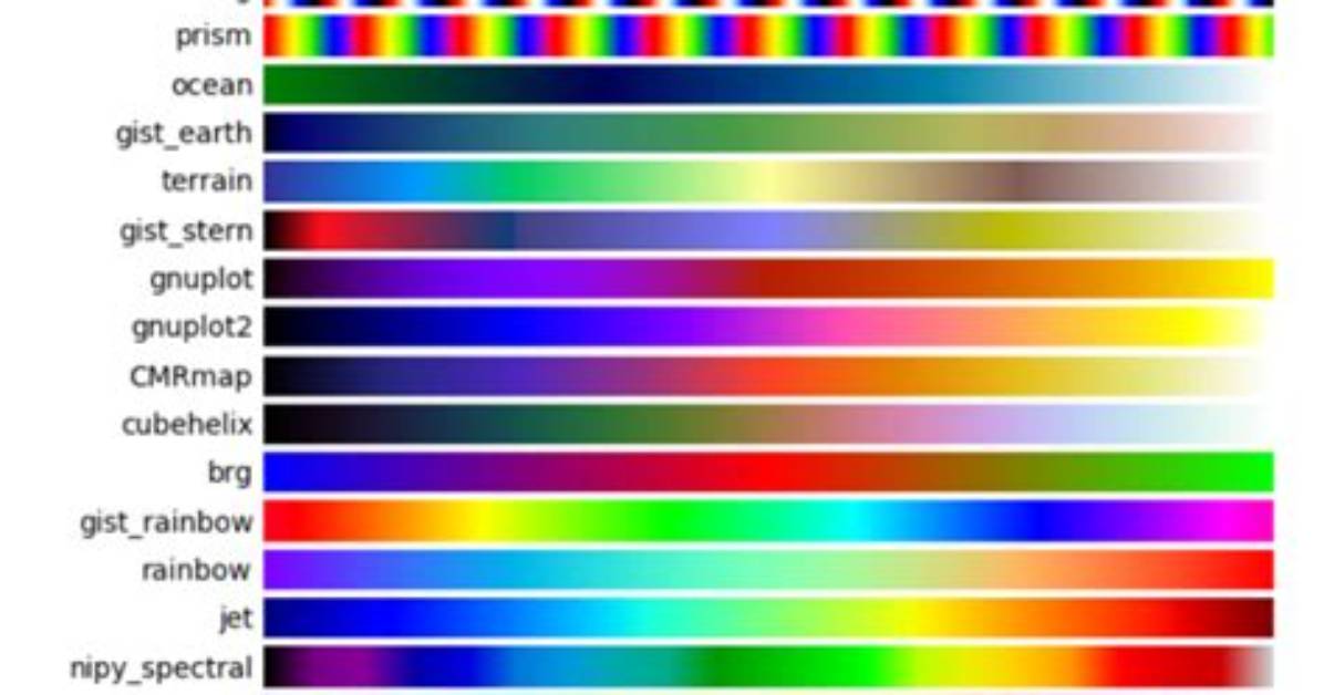
However, if img were an array of shape (M,N), then the cmap controls the colormap used to display the values.
import numpy as np
import matplotlib.pyplot as plt
import mpl_toolkits.axes_grid1 as axes_grid1
np.random.seed(1)

data = np.random.randn(10, 10)

fig = plt.figure()
grid = axes_grid1.AxesGrid(
    fig, 111, nrows_ncols=(1, 2), axes_pad = 0.5, cbar_location = "right",
    cbar_mode="each", cbar_size="15%", cbar_pad="5%",)

im0 = grid[0].imshow(data, cmap='gray', interpolation='nearest')
grid.cbar_axes[0].colorbar(im0)

im1 = grid[1].imshow(data, cmap='jet', interpolation='nearest')
grid.cbar_axes[1].colorbar(im1)
plt.savefig('/tmp/test.png', bbox_inches='tight', pad_inches=0.0, dpi=200,)
David Miller brings 15 years of experience in global economics, personal finance strategy, and market dynamics. He specializes in turning complex economic trends into actionable insights for everyday readers.
