
Sklearn Plot Confusion Matrix with Labels

I Want to Plot a Confusion Matrix to Visualize the Classifer's Performance, but It Shows Only the Numbers of the Labels, Not the Labels Themselves: from...
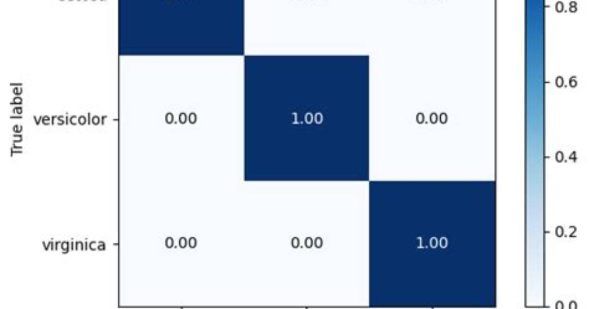
I want to plot a confusion matrix to visualize the classifer's performance, but it shows only the numbers of the labels, not the labels themselves:
from sklearn.metrics import confusion_matrix
import pylab as pl
y_test=['business', 'business', 'business', 'business', 'business', 'business', 'business', 'business', 'business', 'business', 'business', 'business', 'business', 'business', 'business', 'business', 'business', 'business', 'business', 'business']

pred=array(['health', 'business', 'business', 'business', 'business',
       'business', 'health', 'health', 'business', 'business', 'business',
       'business', 'business', 'business', 'business', 'business',
       'health', 'health', 'business', 'health'],
      dtype='|S8')

cm = confusion_matrix(y_test, pred)
pl.matshow(cm)
pl.title('Confusion matrix of the classifier')
pl.colorbar()
pl.show()
How can I add the labels (health, business..etc) to the confusion matrix?
9 Answers
UPDATE:
In scikit-learn 0.22, there's a new feature to plot the confusion matrix directly (which, however, is deprecated in 1.0 and will be removed in 1.2).
See the documentation: sklearn.metrics.plot_confusion_matrix
OLD ANSWER:
I think it's worth mentioning the use of seaborn.heatmap here.
import seaborn as sns
import matplotlib.pyplot as plt

ax= plt.subplot()
sns.heatmap(cm, annot=True, fmt='g', ax=ax);  #annot=True to annotate cells, ftm='g' to disable scientific notation

# labels, title and ticks
ax.set_xlabel('Predicted labels');ax.set_ylabel('True labels');
ax.set_title('Confusion Matrix');
ax.xaxis.set_ticklabels(['business', 'health']); ax.yaxis.set_ticklabels(['health', 'business']);
As hinted in this question, you have to "open" the lower-level artist API, by storing the figure and axis objects passed by the matplotlib functions you call (the fig, ax and cax variables below). You can then replace the default x- and y-axis ticks using set_xticklabels/set_yticklabels:
from sklearn.metrics import confusion_matrix

labels = ['business', 'health']
cm = confusion_matrix(y_test, pred, labels)
print(cm)
fig = plt.figure()
ax = fig.add_subplot(111)
cax = ax.matshow(cm)
plt.title('Confusion matrix of the classifier')
fig.colorbar(cax)
ax.set_xticklabels([''] + labels)
ax.set_yticklabels([''] + labels)
plt.xlabel('Predicted')
plt.ylabel('True')
plt.show()
Note that I passed the labels list to the confusion_matrix function to make sure it's properly sorted, matching the ticks.
This results in the following figure:
I found a function that can plot the confusion matrix which generated from sklearn.
import numpy as np


def plot_confusion_matrix(cm,
                          target_names,
                          title='Confusion matrix',
                          cmap=None,
                          normalize=True):
    """
    given a sklearn confusion matrix (cm), make a nice plot

    Arguments
    ---------
    cm:           confusion matrix from sklearn.metrics.confusion_matrix

    target_names: given classification classes such as [0, 1, 2]
                  the class names, for example: ['high', 'medium', 'low']

    title:        the text to display at the top of the matrix

    cmap:         the gradient of the values displayed from matplotlib.pyplot.cm
                  see
                  plt.get_cmap('jet') or plt.cm.Blues

    normalize:    If False, plot the raw numbers
                  If True, plot the proportions

    Usage
    -----
    plot_confusion_matrix(cm           = cm,                  # confusion matrix created by
                                                              # sklearn.metrics.confusion_matrix
                          normalize    = True,                # show proportions
                          target_names = y_labels_vals,       # list of names of the classes
                          title        = best_estimator_name) # title of graph

    Citiation
    ---------


    """
    import matplotlib.pyplot as plt
    import numpy as np
    import itertools

    accuracy = np.trace(cm) / np.sum(cm).astype('float')
    misclass = 1 - accuracy

    if cmap is None:
        cmap = plt.get_cmap('Blues')

    plt.figure(figsize=(8, 6))
    plt.imshow(cm, interpolation='nearest', cmap=cmap)
    plt.title(title)
    plt.colorbar()

    if target_names is not None:
        tick_marks = np.arange(len(target_names))
        plt.xticks(tick_marks, target_names, rotation=45)
        plt.yticks(tick_marks, target_names)

    if normalize:
        cm = cm.astype('float') / cm.sum(axis=1)[:, np.newaxis]


    thresh = cm.max() / 1.5 if normalize else cm.max() / 2
    for i, j in itertools.product(range(cm.shape[0]), range(cm.shape[1])):
        if normalize:
            plt.text(j, i, "{:0.4f}".format(cm[i, j]),
                     horizontalalignment="center",
                     color="white" if cm[i, j] > thresh else "black")
        else:
            plt.text(j, i, "{:,}".format(cm[i, j]),
                     horizontalalignment="center",
                     color="white" if cm[i, j] > thresh else "black")


    plt.tight_layout()
    plt.ylabel('True label')
    plt.xlabel('Predicted label\naccuracy={:0.4f}; misclass={:0.4f}'.format(accuracy, misclass))
    plt.show()
It will look like this
To add to @akilat90's update about sklearn.metrics.plot_confusion_matrix:
You can use the ConfusionMatrixDisplay class within sklearn.metrics directly and bypass the need to pass a classifier to plot_confusion_matrix. It also has the display_labels argument, which allows you to specify the labels displayed in the plot as desired.
The constructor for ConfusionMatrixDisplay doesn't provide a way to do much additional customization of the plot, but you can access the matplotlib axes obect via the ax_ attribute after calling its plot() method. I've added a second example showing this.
I found it annoying to have to rerun a classifier over a large amount of data just to produce the plot with plot_confusion_matrix. I am producing other plots off the predicted data, so I don't want to waste my time re-predicting every time. This was an easy solution to that problem as well.
Example:
from sklearn.metrics import confusion_matrix, ConfusionMatrixDisplay

cm = confusion_matrix(y_true, y_preds, normalize='all')
cmd = ConfusionMatrixDisplay(cm, display_labels=['business','health'])
cmd.plot()
Example using ax_:
cm = confusion_matrix(y_true, y_preds, normalize='all')
cmd = ConfusionMatrixDisplay(cm, display_labels=['business','health'])
cmd.plot()
cmd.ax_.set(xlabel='Predicted', ylabel='True')
from sklearn import model_selection
test_size = 0.33
seed = 7
X_train, X_test, y_train, y_test = model_selection.train_test_split(feature_vectors, y, test_size=test_size, random_state=seed)

from sklearn.metrics import accuracy_score, f1_score, precision_score, recall_score, classification_report, confusion_matrix

model = LogisticRegression()
model.fit(X_train, y_train)
result = model.score(X_test, y_test)
print("Accuracy: %.3f%%" % (result*100.0))
y_pred = model.predict(X_test)
print("F1 Score: ", f1_score(y_test, y_pred, average="macro"))
print("Precision Score: ", precision_score(y_test, y_pred, average="macro"))
print("Recall Score: ", recall_score(y_test, y_pred, average="macro"))

import numpy as np
import pandas as pd
import matplotlib.pyplot as plt
import seaborn as sns
from sklearn.metrics import confusion_matrix

def cm_analysis(y_true, y_pred, labels, ymap=None, figsize=(10,10)):
    """
    Generate matrix plot of confusion matrix with pretty annotations.
    The plot image is saved to disk.
    args:
      y_true:    true label of the data, with shape (nsamples,)
      y_pred:    prediction of the data, with shape (nsamples,)
      filename:  filename of figure file to save
      labels:    string array, name the order of class labels in the confusion matrix.
                 use `clf.classes_` if using scikit-learn models.
                 with shape (nclass,).
      ymap:      dict: any -> string, length == nclass.
                 if not None, map the labels & ys to more understandable strings.
                 Caution: original y_true, y_pred and labels must align.
      figsize:   the size of the figure plotted.
    """
    if ymap is not None:
        y_pred = [ymap[yi] for yi in y_pred]
        y_true = [ymap[yi] for yi in y_true]
        labels = [ymap[yi] for yi in labels]
    cm = confusion_matrix(y_true, y_pred, labels=labels)
    cm_sum = np.sum(cm, axis=1, keepdims=True)
    cm_perc = cm / cm_sum.astype(float) * 100
    annot = np.empty_like(cm).astype(str)
    nrows, ncols = cm.shape
    for i in range(nrows):
        for j in range(ncols):
            c = cm[i, j]
            p = cm_perc[i, j]
            if i == j:
                s = cm_sum[i]
                annot[i, j] = '%.1f%%\n%d/%d' % (p, c, s)
            elif c == 0:
                annot[i, j] = ''
            else:
                annot[i, j] = '%.1f%%\n%d' % (p, c)
    cm = pd.DataFrame(cm, index=labels, columns=labels)
    cm.index.name = 'Actual'
    cm.columns.name = 'Predicted'
    fig, ax = plt.subplots(figsize=figsize)
    sns.heatmap(cm, annot=annot, fmt='', ax=ax)
    #plt.savefig(filename)
    plt.show()

cm_analysis(y_test, y_pred, model.classes_, ymap=None, figsize=(10,10))
using
Note that if you use rocket_r it will reverse the colors and somehow it looks more natural and better such as below:
You might be interested by
which implements a Python Pandas implementation of Confusion Matrix.
Some features:
- plot confusion matrix
- plot normalized confusion matrix
- class statistics
- overall statistics
Here is an example:
In [1]: from pandas_ml import ConfusionMatrix
In [2]: import matplotlib.pyplot as plt

In [3]: y_test = ['business', 'business', 'business', 'business', 'business',
        'business', 'business', 'business', 'business', 'business',
        'business', 'business', 'business', 'business', 'business',
        'business', 'business', 'business', 'business', 'business']

In [4]: y_pred = ['health', 'business', 'business', 'business', 'business',
       'business', 'health', 'health', 'business', 'business', 'business',
       'business', 'business', 'business', 'business', 'business',
       'health', 'health', 'business', 'health']

In [5]: cm = ConfusionMatrix(y_test, y_pred)

In [6]: cm
Out[6]:
Predicted  business  health  __all__
Actual
business         14       6       20
health            0       0        0
__all__          14       6       20

In [7]: cm.plot()
Out[7]: <matplotlib.axes._subplots.AxesSubplot at 0x1093cf9b0>

In [8]: plt.show()
In [9]: cm.print_stats()
Confusion Matrix:

Predicted  business  health  __all__
Actual
business         14       6       20
health            0       0        0
__all__          14       6       20


Overall Statistics:

Accuracy: 0.7
95% CI: (0.45721081772371086, 0.88106840959427235)
No Information Rate: ToDo
P-Value [Acc > NIR]: 0.608009812201
Kappa: 0.0
Mcnemar's Test P-Value: ToDo


Class Statistics:

Classes                                 business health
Population                                    20     20
P: Condition positive                         20      0
N: Condition negative                          0     20
Test outcome positive                         14      6
Test outcome negative                          6     14
TP: True Positive                             14      0
TN: True Negative                              0     14
FP: False Positive                             0      6
FN: False Negative                             6      0
TPR: (Sensitivity, hit rate, recall)         0.7    NaN
TNR=SPC: (Specificity)                       NaN    0.7
PPV: Pos Pred Value (Precision)                1      0
NPV: Neg Pred Value                            0      1
FPR: False-out                               NaN    0.3
FDR: False Discovery Rate                      0      1
FNR: Miss Rate                               0.3    NaN
ACC: Accuracy                                0.7    0.7
F1 score                               0.8235294      0
MCC: Matthews correlation coefficient        NaN    NaN
Informedness                                 NaN    NaN
Markedness                                     0      0
Prevalence                                     1      0
LR+: Positive likelihood ratio               NaN    NaN
LR-: Negative likelihood ratio               NaN    NaN
DOR: Diagnostic odds ratio                   NaN    NaN
FOR: False omission rate                       1      0
    from sklearn.metrics import confusion_matrix
    import seaborn as sns
    import matplotlib.pyplot as plt
    model.fit(train_x, train_y,validation_split = 0.1, epochs=50, batch_size=4)
    y_pred=model.predict(test_x,batch_size=15)
    cm =confusion_matrix(test_y.argmax(axis=1), y_pred.argmax(axis=1))
    index = ['neutral','happy','sad']
    columns = ['neutral','happy','sad']
    cm_df = pd.DataFrame(cm,columns,index)
    plt.figure(figsize=(10,6))
    sns.heatmap(cm_df, annot=True)
There is a very easy way to do this using ConfusionMatrixDisplay. It supports display_labels which can be used to display labels for plot
import numpy as np
from sklearn.metrics import confusion_matrix, ConfusionMatrixDisplay
np.random.seed(0)
y_true = np.random.randint(0,3, 100)
y_pred = np.random.randint(0,3, 100)

labels = ['cat', 'dog', 'rat']

cm = confusion_matrix(y_true, y_pred)
ConfusionMatrixDisplay(cm, display_labels=labels).plot()
#plt.savefig("Confusion_Matrix.png")
Output:
Given model, validx, validy. With great help from other answers, this is what fits my needs.
sklearn.metrics.plot_confusion_matrix
import matplotlib.pyplot as plt
fig, ax = plt.subplots(figsize=(26,26))
sklearn.metrics.plot_confusion_matrix(model, validx, validy, ax=ax, cmap=plt.cm.Blues)
ax.set(xlabel='Predicted', ylabel='Actual', title='Confusion Matrix Actual vs Predicted')
James Sterling reports on renewable energy developments, climate policy, ecological conservation, and green tech innovations around the globe.
