
Integrating Factor in Differential Equation

In the Context of Solving Ordinary Differential Equations (Odes), an Integrating Factor Is a Function That Can Be Multiplied with the Entire Ode to Make It...
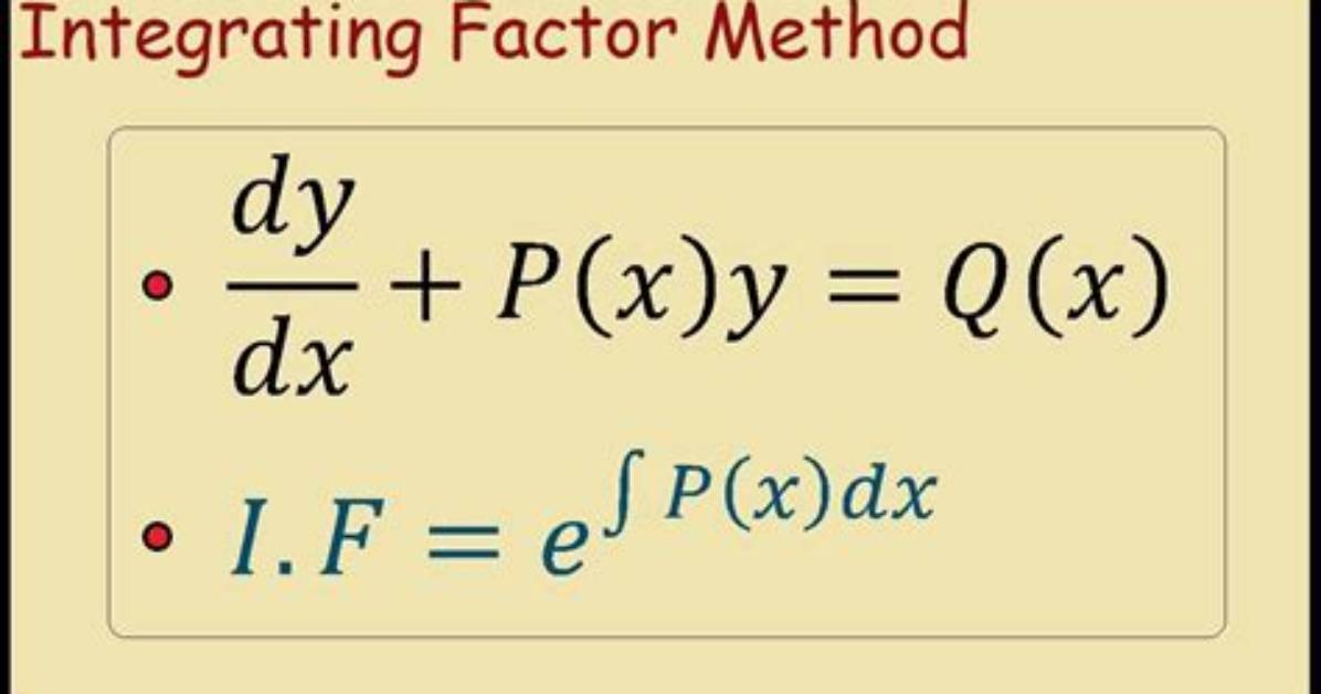
In the context of solving ordinary differential equations (ODEs), an integrating factor is a function that can be multiplied with the entire ODE to make it exact. Exact ODEs are easier to solve because they can be written as the total differential of some function, which makes it possible to find an analytical solution.
Here's the general approach for using an integrating factor to solve an ODE:
-
Write the ODE in standard form:
M(x, y)dx + N(x, y)dy = 0
where M and N are functions of the independent variable x and the dependent variable y.
-
Check if the ODE is exact: An ODE is exact if the following condition is satisfied:
∂M/∂y = ∂N/∂x
If the ODE is already exact, you can proceed to solve it directly. If it's not exact, you'll need to find an integrating factor.
-
Find the integrating factor (IF): The integrating factor, denoted as μ(x, y), is a function that can be used to make the ODE exact. It is found by solving the following equation:
μ(x, y) = 1 / (IF condition) = 1 / ((∂M/∂y - ∂N/∂x) / N)
-
Multiply the entire ODE by the integrating factor:
μ(x, y) [M(x, y)dx + N(x, y)dy] = 0
-
Check if the new ODE is exact: Multiply out and rearrange the equation to see if it can be expressed as the total differential of some function. The transformed ODE should have the form:
dF(x, y) = 0
where F(x, y) is the function you're trying to find.
-
Integrate to find the solution: If the transformed ODE is exact, you can find the solution by integrating the total differential equation with respect to x or y, depending on the form of the equation.
-
Don't forget to include any initial conditions if they are given.
The integrating factor method is a powerful tool for solving first-order ODEs that are not exact. It transforms the ODE into an exact one, making it easier to find a solution. Keep in mind that finding the right integrating factor can sometimes be challenging, and it may not always be straightforward, but it is a valuable technique in solving ODEs.
What are Differential Equations?
Differential equations are mathematical equations that involve one or more derivatives of an unknown function. These equations describe how a function changes as a result of the rates of change of its variables. They are widely used in various fields of science and engineering to model and analyze dynamic systems and processes.
Differential equations can be classified into several categories based on their properties and characteristics:
-
Ordinary Differential Equations (ODEs): These equations involve a single independent variable, such as time, and its derivatives with respect to that variable. ODEs are often used to describe the behavior of a single variable over time, like the motion of a particle, population growth, or electrical circuits.
-
Partial Differential Equations (PDEs): PDEs involve multiple independent variables and their partial derivatives. They are used to describe systems where the unknown function depends on multiple variables, such as temperature distribution in a solid, fluid flow, or electromagnetic field propagation.
-
Linear Differential Equations: Linear differential equations are equations where the unknown function and its derivatives appear in a linear manner. Solving linear differential equations is often more straightforward and well-understood than nonlinear ones.
-
Nonlinear Differential Equations: Nonlinear differential equations involve the unknown function and its derivatives in a nonlinear manner. These equations are more challenging to solve and can exhibit complex and chaotic behavior.
Differential equations are essential in various scientific and engineering disciplines, including physics, chemistry, biology, economics, and engineering. They provide a powerful tool for modeling and understanding dynamic systems and predicting their future behavior. Solutions to differential equations can take various forms, depending on the equation's order and type, and can be expressed as explicit functions, implicit relationships, or as numerical approximations using computational methods. Solving differential equations plays a crucial role in scientific research, technology development, and real-world applications.
Must Read
Integrating Factor Method
The integrating factor method is a technique used to solve first-order linear ordinary differential equations. These are differential equations of the form:
dy/dx + P(x)y = Q(x)
In this equation, y is the dependent variable, x is the independent variable, and P(x) and Q(x) are functions of x.
The integrating factor method involves multiplying the entire equation by an integrating factor, which is a function of x. The goal is to transform the given equation into a form that allows for easier integration and the solution of the differential equation.
Here are the steps to solve a first-order linear ODE using the integrating factor method:
-
Identify the coefficients P(x) and Q(x) in the equation dy/dx + P(x)y = Q(x).
-
Determine the integrating factor (IF), denoted by μ(x), which is a function of x and is chosen in such a way that when you multiply the entire equation by μ(x), it becomes an exact differential equation. The integrating factor is typically calculated as μ(x) = e^(∫P(x)dx), where ∫P(x)dx represents the integral of P(x) with respect to x.
-
Multiply the original differential equation by the integrating factor μ(x):
μ(x) * (dy/dx + P(x)y) = μ(x) * Q(x)
This transforms the equation into:
μ(x) * dy/dx + μ(x) * P(x)y = μ(x) * Q(x)
- The left side of the equation, μ(x) * dy/dx + μ(x) * P(x)y, is now an exact differential, and you can write it as the derivative of a product:
d(μ(x)y)/dx = μ(x) * Q(x)
- Integrate both sides of the equation with respect to x:
∫d(μ(x)y)/dx dx = ∫μ(x) * Q(x) dx
- Integrate the left side to obtain μ(x)y, and integrate the right side to obtain the antiderivative of μ(x) * Q(x):
μ(x)y = ∫μ(x) * Q(x) dx + C
- Solve for y:
y = (1/μ(x)) * (∫μ(x) * Q(x) dx + C)
- Simplify the right side of the equation and, if necessary, solve for C using initial conditions if provided.
This is the general procedure for using the integrating factor method to solve first-order linear ordinary differential equations. The choice of the integrating factor μ(x) simplifies the equation and allows for easier integration to find the solution.
David Miller brings 15 years of experience in global economics, personal finance strategy, and market dynamics. He specializes in turning complex economic trends into actionable insights for everyday readers.
